Dynamic Sorted Lists

Dynamic Alphabetical Sorting in Excel

In this guide, we’ll explore how to maintain an alphabetically sorted list of names in Excel, even as new data is added. This process involves creating a dynamic model that updates automatically. Let's walk through the steps:

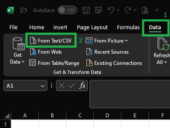
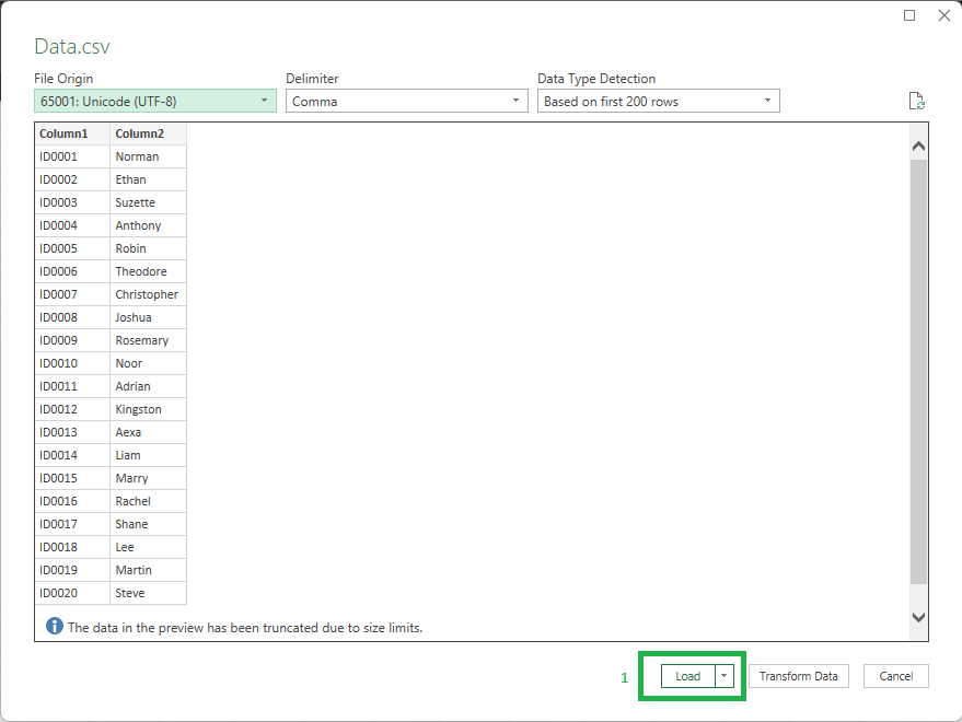
STEP 1: Load Data into Excel

Start by importing your data into Excel. In this example, we’ll load data from a local file, but in real-world applications, you might pull data directly from a database. Ensure that your data is organized in a tabular format, with clear headers for each column (e.g., "Name," "Employee ID," etc.).

STEP 2: Get Row Number

To facilitate sorting and referencing, we’ll add a column to capture the row number of each entry.

1. Ensure your headers are clear and descriptive.
2. Add a new column titled "Row Number." In the first cell of this column (assuming it's the first row of your data), enter the following formula:

 =ROW([@Row])-ROW(Data[[#Headers],[Row]])

Above formula calculates the row number of each entry by subtracting the row number of the header from the current row. The cell references [@Row] and [[#Headers],[Row]] are automatically generated by Excel when you select a cell, allowing for dynamic updates regardless of the table's position.

STEP 3: Create Rank

Next, we’ll create another column to rank the names alphabetically.

1. Add another column named "Rank."
2. In the first cell under "Rank," use the following formula:

=COUNTIF([First Name],"<="&[@[First Name]])

Rank formula counts how many names are less than or equal to the current name in alphabetical order, effectively giving each name its rank.

STEP 4: Create a Dynamic List

Now, we will create a dynamic list that updates automatically as new data is added.

=INDEX([Name], MATCH(ROW()-ROW(StartCell)+1, [Rank], 0))

Above formula pulls names based on their rank, ensuring the list remains in alphabetical order.

Use Case of Dynamic Sorted List: A Dropdown List

Let’s create a dropdown menu that allows users to select an employee and pull respective ID. Employee names should always be in alphabetic order.

• Select the range of your dynamic list and give it a name (e.g., "NamedList").

• Go to the cell where we want the dropdown to appear, and navigate to Data > Data Validation, then choose "List" and set the source to the named range.

• Retrieve the corresponding Employee ID based on the selected name using the INDEX and MATCH functions in the adjacent cell:

=INDEX([Employee ID], MATCH(SelectedCell, [Name], 0))

• Lets add another employee to the list and see the result.

Conclusion

By following these steps, we successfully created a dynamic model in Excel that maintains alphabetical order for names, allows for easy data entry, and enhances user interaction through dropdown menus. This model is robust and adaptable, ensuring that your data remains organized and accessible as new entries are added.