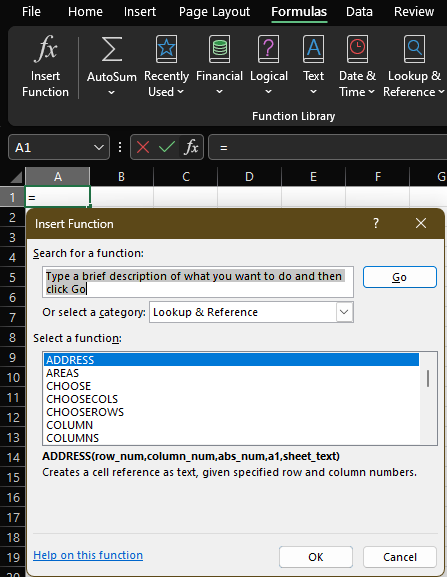
Lookup and reference functions are used to reference another cell, range, or table in the same or another worksheet or workbook. The functions covered in this article are not an exhaustive list but focus on those most likely to be used in financial and accounting dashboards and models.
VLOOKUP
The VLOOKUP function is one of the simplest and most commonly used functions to reference data in another cell, range, or table.
VLOOKUP(lookup_value, table_array, col_index_num, [range_lookup])
| Argument | Description |
lookup_value | What to look for, in our example it is the country in cell C14. |
table_array | Where to look for values, in our example it is the table named t_captains. If data is not in a table or a named range, then cells can be referenced such as A3:D12. |
col_index_num | This is the result we are looking for; we need to specify the column number to reference the data. |
[rangelookup] | Optional logical argument (TRUE or FALSE) to indicate whether approximate values should be matched. In most cases we would specify FALSE to only match exact values. |
Example:
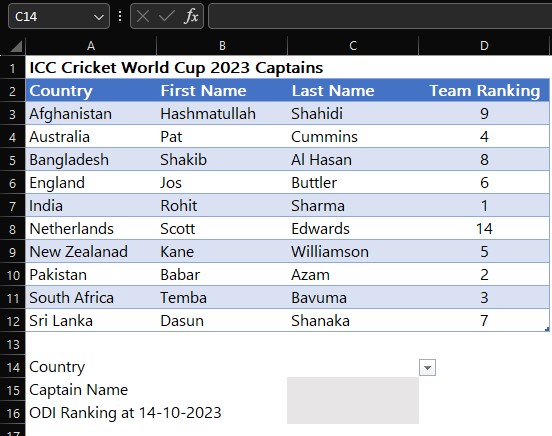
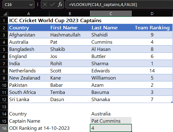
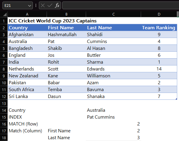
Based on the country selected in the dropdown in cell C14, we need Captain's full name in cell C15 and ODI ranking for the country in cell C16 from the data table.
C15: =VLOOKUP(c14,t_captains,2,FALSE)&" "&=VLOOKUP(c14,t_captains,3,FALSE)
C16: =VLOOKUP(c14,t_captains,4,FALSE)
Notes:
- VLOOKUP searches for the lookup value in the first column of the specified table array, making this function useful only if the lookup values are in the first column of the data.
- Lookup values must be sorted; in this case, country names should be alphabetically sorted.
- Lookup values must be unique without duplication.
HLOOKUP
HLOOKUP is similar to VLOOKUP but is used when data is organized in rows rather than columns.
HLOOKUP(lookup_value, table_array, row_index_num, [rangelookup])
Due to the limitations of VLOOKUP and HLOOKUP, other lookup functions such as XLOOKUP and INDEX-MATCH are often better options, though they may be more complex.
XLOOKUP
XLOOKUP is a new, more flexible, and powerful function that serves as a great alternative to VLOOKUP and HLOOKUP.
XLOOKUP(lookup_value, lookup_array, return_array, [if not found], [match mode], [search_mode])
| Argument | Description |
lookup_value | Value to match, in our example it is the country name in cell C8 |
lookup_array | Where to lookup, in our example this would be the countries row (or column if the data was columnar) |
return_array | Rows or columns that contains required data, in our example it is row 3 to 6 containing first name, last name and team ranking. |
| [if not found] | Optional argument; to return specified result if no matching value is found in lookup array. |
| [match mode] | Optional argument. To specify exact or wildcard match etc. |
[search mode] | Optional argument. Can specify how excel performs the search for example ascending, descending etc. |
Example:
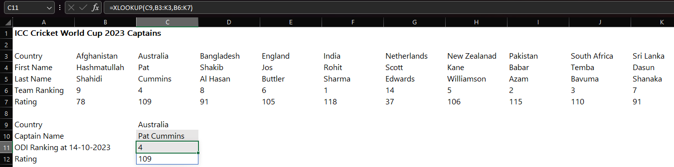
We need the team captain's full name and country ranking, but this time the data is in columnar format.
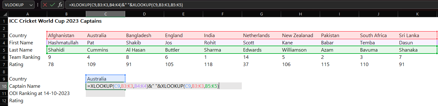
C10: =XLOOKUP(C9,B3:K3,B4:K4)&" "&XLOOKUP(C9,B3K3,B5:K5)
XLOOKUP can also return values from multiple rows or columns. Below, we retrieve results as an array from the formula in cell C11.
=XLOOKUP(C9,B3:K3,B6:K7)
INDEX & MATCH
Although INDEX and MATCH are separate Excel functions, they are often combined to look up values.
INDEX(array, row_num, [coulmn_num]
INDEX requires a row number and column number to retrieve the desired result. This is where the MATCH function comes in; instead of hardcoding row and column values, we can dynamically determine these using MATCH.
MATCH(lookup_value, lookup_array, [match_type])
Example:
Continuing with the previous example, let's get the captain's full name and ODI ranking. We will first retrieve the values individually using INDEX and MATCH and then combine them.
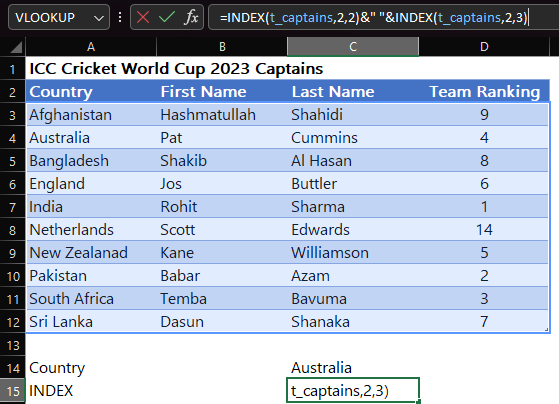
C15: =INDEX(t_captains,2,2)&" "&INDEX(t_captains,2,3)
Hardcoding row and column numbers for each lookup is not recommended. Instead, let's reference values in A14 and A15.
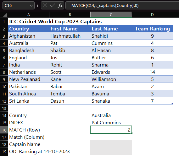
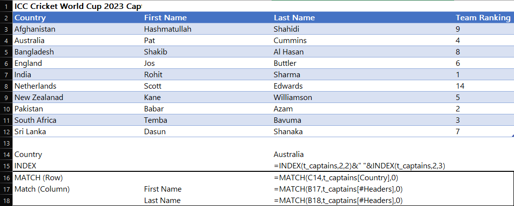
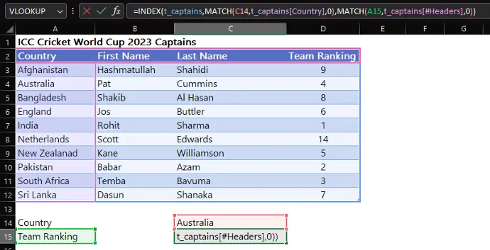
Combined INDEX and MATCH Formula in C15:
INDEX(t_captains,MATCH(C14,t_captains[country],0),MATCH(A15,t_captains[#Headers],0))
Note: In most cases it is sufficient to use INDEX-MATCH for rows only.
UNIQUE
As the name suggests, the UNIQUE function retrieves unique values from a list.
UNIQUE(array, [by_col], [exactly once])
Argument | Description |
array | This is the name of array, in our example it is the Unique Customer and unique Region columns. |
[by_col] | Logical TRUE FALSE argument to specify whether to return unique values in rows or columns, We require unique rows so our input is FALSE |
[exactly_once] | Logical TRUE FALSE argument to specify if unique value is the one that occurs only once is required. In our example it is FALSE. |
Example:
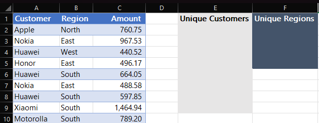
We have a list of sales data in a table named `t_sales` with customer names and regions, and we want to extract unique customer names and regions in columns E and F, respectively.
We get unique customers and regions in columns E and F respectively.
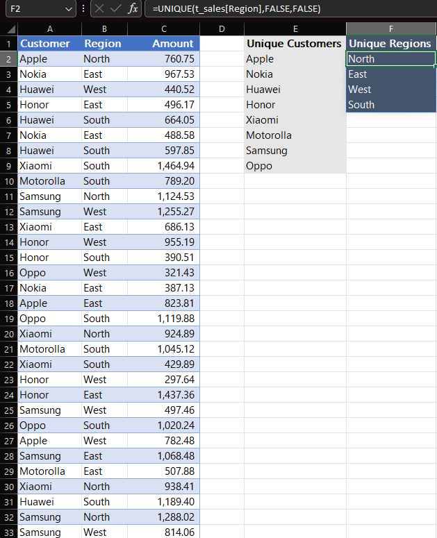
E2: =UNIQUE(t_sales[Customer], FALSE, FALSE)
F2: =UNIQUE(t_sales[Region], FALSE, FALSE)
OFFSET
The OFFSET function returns a cell or range reference that is a specified number of rows or columns away from a given cell or range.
OFFSET(reference, rows, cols, [height], [width])
| Argument | Description |
reference | This is the cell original formula would refer to if there was no offset, for gross profit percentage it is cell B9 and for net profit percentage it is B10. (First value in the relevant row or column) |
rows | number of rows to offset. In our example as our data is columnar meaning we need data from the same row, there is no need to offset row therefore our input is 0 |
col | Number of columns to offset. This is what we require. We reference cell B12 and subtract 1 to get correct number of columns to offset. |
| [height] | Optional argument to specify how many rows to output. In our example we only need the result in a single cell and not a range, so this argument is omitted. |
| [width] | Optional argument to specify how many columns to output. In our example we only need the result in a single cell and not a range, so this argument is omitted. |
Example:
We have a twelve-month income statement, and we need gross profit and net profit percentages in cells C13 and C14, respectively, based on the month selected in the dropdown in cell B12.
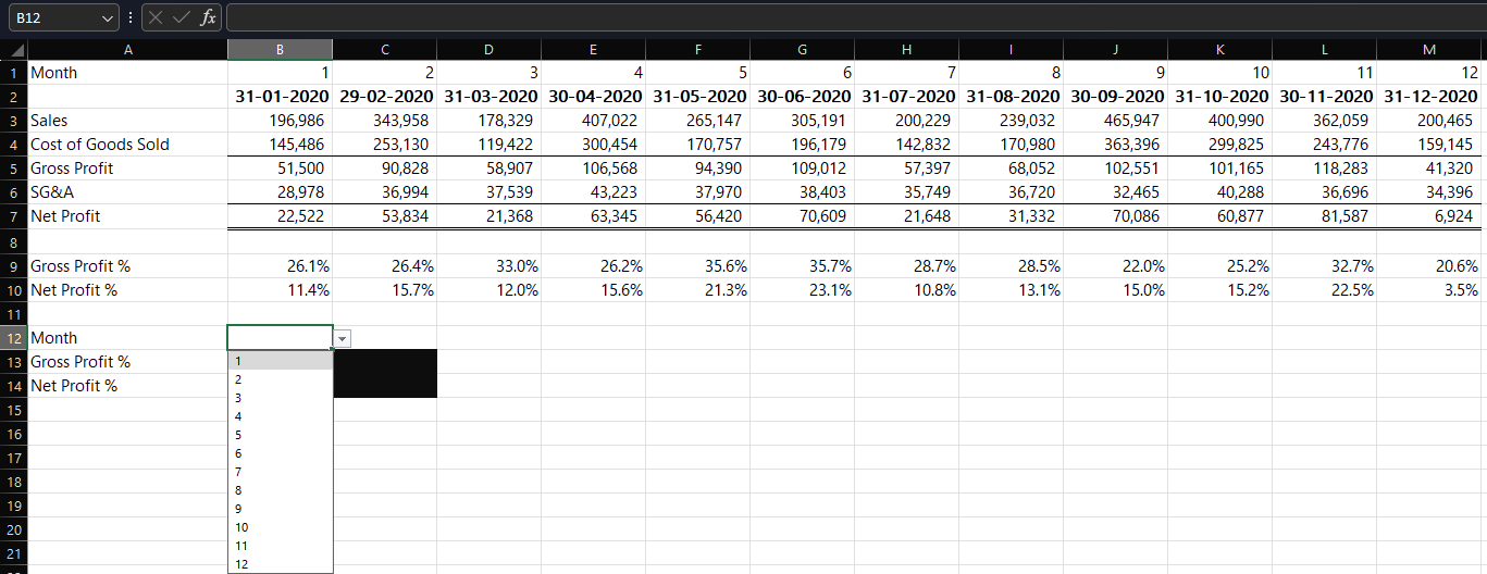
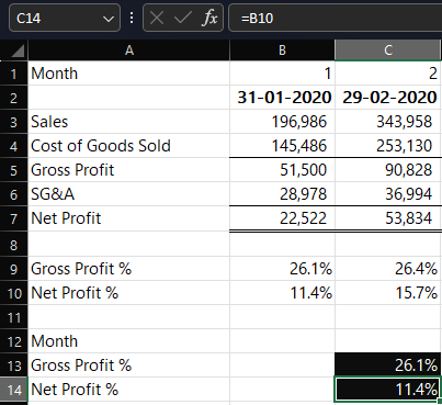
Lets begin by referencing gross profit and net profit and net profit percentages for month 1 in C13 & C14.
Next lets use offset to get values based on month selected in cell C12.
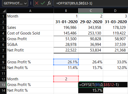
C13: =OFFSET(B9, 0, $B$12 - 1)
C14: =OFFSET(B10, 0, $B$12 - 1)
When the month is changed in B12, the gross profit and net profit percentages for that month are displayed accordingly.
ROW
The ROW function returns the row number of a reference.
ROW([reference])
Example:
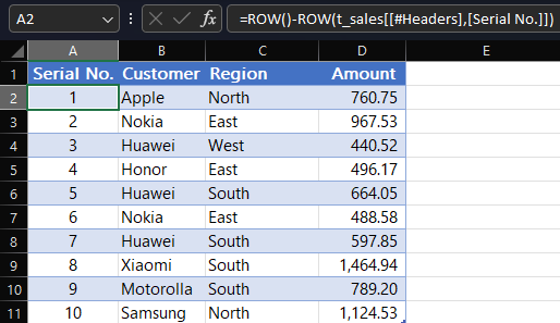
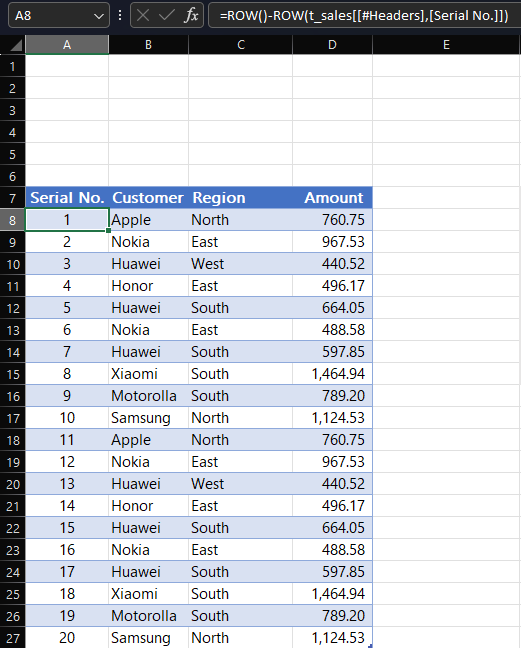
We need a dynamic serial number column in the `t_sales` table that updates correctly, even if the table is moved or new data is added.
column A: =ROW() - ROW(t_sales[[#Headers], [Serial No.]])
The first ROW function in this formula returns the row number of the cell containing the formula, while the second ROW function returns the row number of the header. This ensures that the numbering remains consistent, even if the table is relocated.
If we add more lines to the data and insert new rows above the table, the serial numbers will update dynamically, reflecting the new data while maintaining the correct order.
Conclusion
This article covers the most useful lookup and reference functions for accounting and financial models and dashboards.